How To Determine Missing Values In Excel

25 Sep, 2021

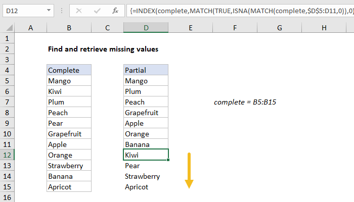
Find and retrieve missing values. One way to find missing values in a list is to use the COUNTIF Function together with the IF Function.

How To Compare Two Columns For Highlighting Missing Values In Excel

An easy method to fill the missing values in excel is to make use of the Go to special option.

How to determine missing values in excel. Of Count Missing Values in Excel. Select the cell B2 and drag the fill handle over the range of cells that you want to contain this formula. IF COUNTIF list cell_value Is there Missing Explanation.

October 2 2016. COUNTIF function keeps the count of cell_value in the list and returns the number to the IF function. Missing values from a list can be checked by using the COUNTIF function passed as a logical test to the IF function.

If there is no missing numbers this formula will return nothing. 1996- 250 1997- 272. FunctionFormula to calculate missing values.

You dont have to worry about the maximum number at which the series ends because the MAX function will automatically take care of that. In the Compare Ranges dialog box you need to. If missing numbers exist it will return the text of Missing in active cell.

INDEX completeMATCHTRUEISNAMATCH complete partial_expanding00 Summary. SUMPRODUCT function returns the sum of TRUE values as 1 and FALSE values as 0 in the array. Click in the Special button.

We will need to test if we find an error NA or not. We start our formula with the IF Function which will test if a condition is met returning one value for TRUE and another for FALSE. Missing columns on excel spreadsheet.

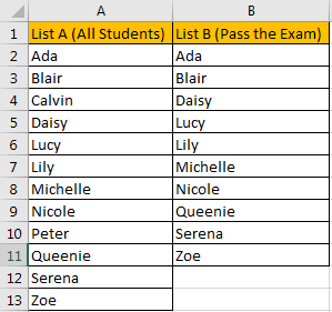
To compare two lists and pull missing values from one list to the other you can use an array formula based on INDEX and MATCH. MATCH finds the position of an item in a list and will return the NA error when a value is not found. How to find missing values in Excel - Excelchat.

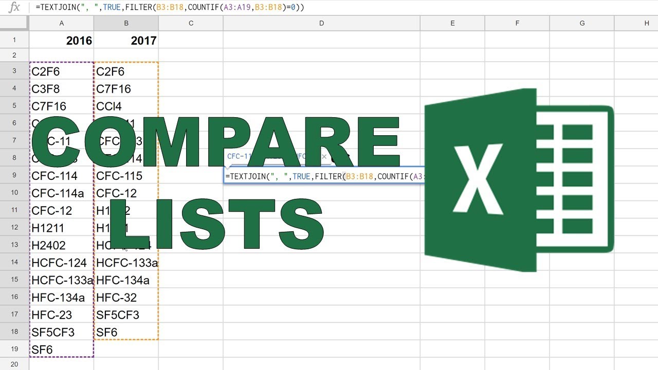
Use the generic formula. TEXTJOIN TRUEFILTERB3B18COUNTIFA3A19B3B180Use the COUNTIF formula to compare 2 lists and find all the values that are in one list but not i. If the value is not found in list COUNTIF returns zero 0 which evaluates as FALSE and IF returns Missing.

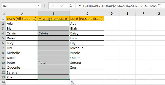
In this tutorial we will help you to find out missing values via two ways the first one is by Conditional Formatting function in excel the second one is by using formula with VLOOKUP function. I am trying to find out how to calculate a missing value based on two or more other values. Imputing the values for missing data Some techniques for imputing values for missing data include.

You can also test for missing values using the MATCH function. Select the rows and columns to be filled. I would like to estimate the values for 1998.

Excel returns 1 data value Osborne as missing from our list1. Step 2 Copy the formula in cell C1 to. Firstly the COUNTIF function takes each values one by one in criteria range and checks it in the range provided.

After the logical test if the entry is found then a string OK is returned otherwise Missing is returned. IFCOUNTIFB3B7D3YesMissing Lets see how this formula works. Copy the formula syntax in cell F2 above and enter it into the remaining cells in column F MISSING to get our desired results.

Find Missing Values. Starting With The IF Function. We will construct a formula out of it.

IF function consider 0 as FALSE and any other integer other than 0 as TRUE. To find the missing values from a list define the value to check for and the list to be checked inside a COUNTIF statement. Substituting the missing data with another observation which is considered similar either taken from another sample or from a previous study Using the.

Now press CtrlG to open the Got to dialog box. If the value is found in the list then the COUNTIF statement returns the numerical value which represents the number of times the value occurs in that list. Click the Kutools Select Select Same Different Cells to open the Compare Ranges dialog box.

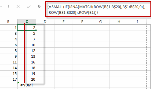
The cell reference in the ROW A1 part of the formula is relative so as you copy the formula down column C ROW A1 becomes ROW A2 which 2 and returns the second smallest missing number ROW A3 which is 3 returns the third smallest missing number and so on. Excel Questions. Find The Missing Values In Excel.

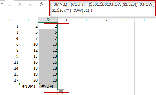
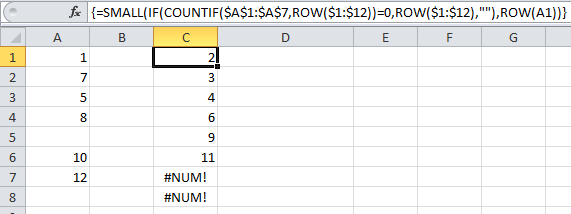
Also its an array formula so press CtrlShiftEnter after entering the formula. Functions Used in this Formula.

How To Identify Missing Numbers Sequence In Excel